Structured Point Clouds (SPCs)
Structured Point Clouds (SPC) is a sparse octree-based representation that is useful to organize and compress 3D geometrically sparse information. They are also known as sparse voxelgrids, quantized point clouds, and voxelized point clouds.
Kaolin supports a number of operations to work with SPCs, including efficient ray-tracing and convolutions.
The SPC data structure is very general. In the SPC data structure, octrees provide a way to store and efficiently retrieve coordinates of points at different levels of the octree hierarchy. It is also possible to associate features to these coordinates using point ordering in memory. Below we detail the low-level representations that comprise SPCs and allow corresponding efficient operations. We also provide a convenience container for these low-level attributes.
Some of the conventions are also defined in Neural Geometric Level of Detail: Real-time Rendering with Implicit 3D Surfaces which uses SPC as an internal representation.
Warning
Structured Point Clouds internal layout and structure is still experimental and may be modified in the future.
Octree
Core to SPC is the octree, a tree data structure where each node have up to 8 childrens. We use this structure to do a recursive three-dimensional space partitioning, i.e: each node represents a partitioning of its 3D space (partition) of \((2, 2, 2)\). The octree then contains the information necessary to find the sparse coordinates.
In SPC, a batch of octrees is represented as a tensor of bytes. Each bit in the byte array octrees represents
the binary occupancy of an octree bit sorted in Morton Order.
The Morton order is a type of space-filling curve which gives a deterministic ordering of
integer coordinates on a 3D grid. That is, for a given non-negative 1D integer coordinate, there exists a
bijective mapping to 3D integer coordinates.
Since a byte is a collection of 8 bits, a single byte octrees[i]
represents an octree node where each bit indicate the binary occupancy of a child node / partition as
depicted below:
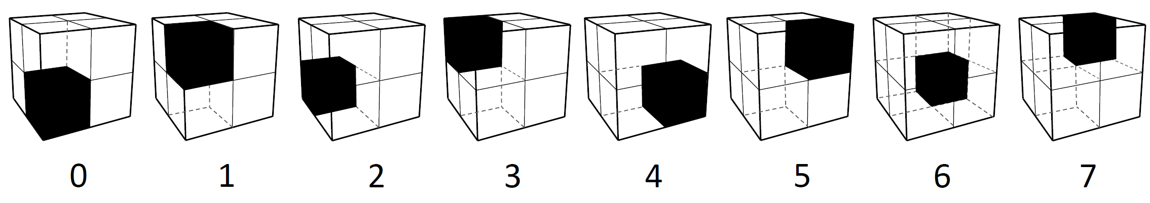
For each octree, the nodes / bytes are following breadth-first-search order (with Morton order for
childrens order), and the octree bytes are then Packed to form octrees. This ordering
allows efficient tree access without having to explicilty store indirection pointers.
The binary occupancy values in the bits of octrees implicitly encode position data due to the bijective
mapping from Morton codes to 3D integer coordinates. However, to provide users a more straight
forward interface to work with these octrees, SPC provides auxilary information such as
points which is a Packed tensor of 3D coordinates. Refer to the Related attributes section
for more details.
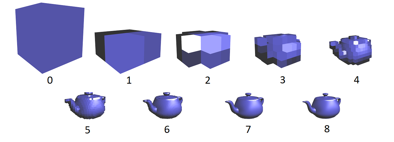
Currently SPCs are primarily used to represent 3D surfaces,
and so all the leaves are at the same level (depth).
This allow very efficient processing on GPU, with custom CUDA kernels, for ray-tracing and convolution.
The structure contains finer details as you go deeper in to the tree. Below are the Levels 0 through 8 of a SPC teapot model:
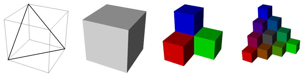
Additional Feature Data
The nodes of the octrees can contain information beyond just the 3D coordinates of the nodes,
such as RGB color, normals, feature maps, or even differentiable activation maps processed by a
convolution.
We follow a Structure of Arrays approach to store
additional data for maximum user extensibility.
Currently the features would be tensors of shape \((\text{num_nodes}, \text{feature_dim})\)
with num_nodes being the number of nodes at a specific level of the octrees,
and feature_dim the dimension of the feature set (for instance 3 for RGB color).
Users can freely define their own feature data to be stored alongside SPC.
Conversions
Structured point clouds can be derived from multiple sources.
We can construct octrees
from unstructured point cloud data, from sparse voxelgrids
or from the level set of an implicit function \(f(x, y, z)\).
Related attributes
Note
If you just wanna use the structured point clouds without having to go through the low level details, take a look at the high level classes.
lengths:
Since octrees use Packed batching, we need lengths a 1D tensor of size batch_size that contains the size of each individual octree. Note that lengths.sum() should equal the size of octrees. You can use kaolin.ops.batch.list_to_packed() to pack octrees and generate lengths
pyramids:
torch.IntTensor of shape \((\text{batch_size}, 2, \text{max_level} + 2)\). Contains layout information for each octree pyramids[:, 0] represent the number of points in each level of the octrees, pyramids[:, 1] represent the starting index of each level of the octree.
exsum:
torch.IntTensor of shape \((\text{octrees_num_bytes} + \text{batch_size})\) is the exclusive sum of the bit counts of each octrees byte.
Note
To generate pyramids and exsum see kaolin.ops.spc.scan_octrees()
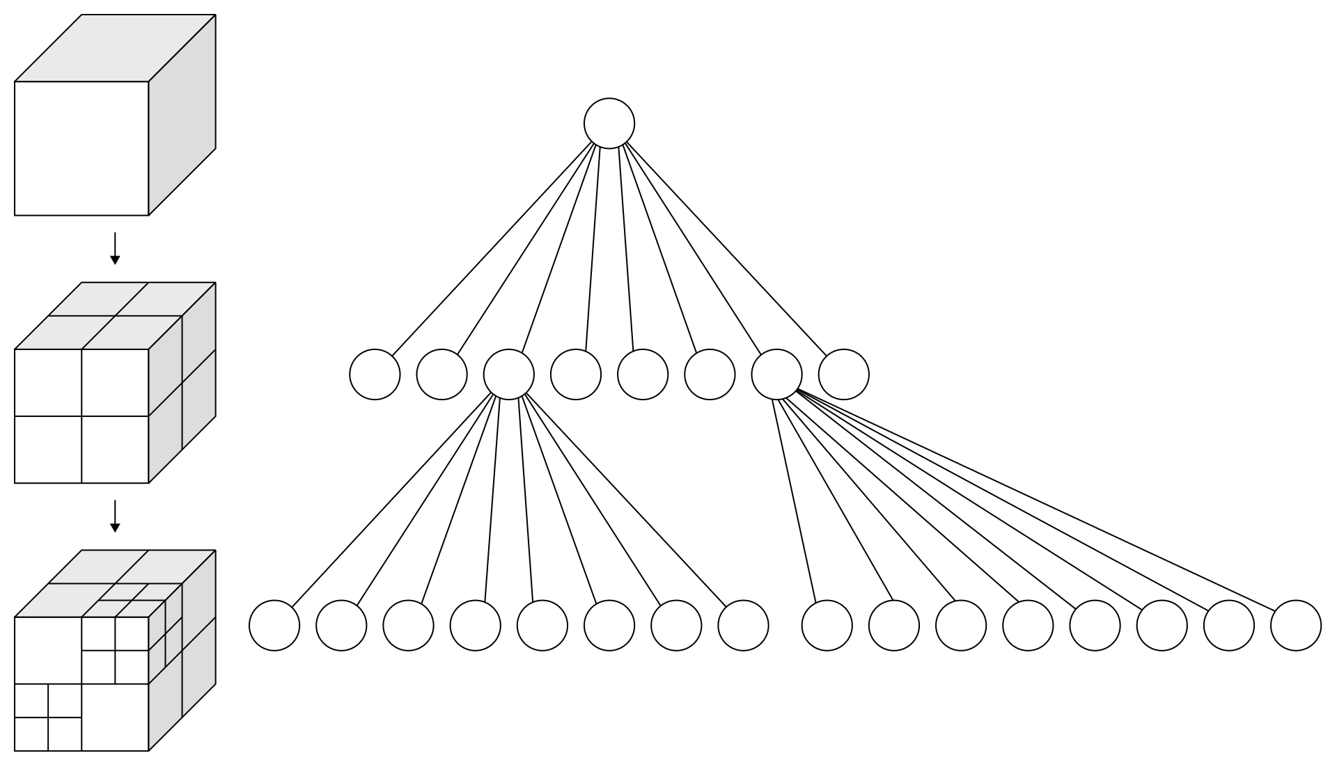
point_hierarchies:
torch.ShortTensor of shape \((\text{num_nodes}, 3)\) correspond to the sparse coordinates at all levels. We refer to this Packed tensor as the structured point hierarchies.
The image below show an analogous 2D example.
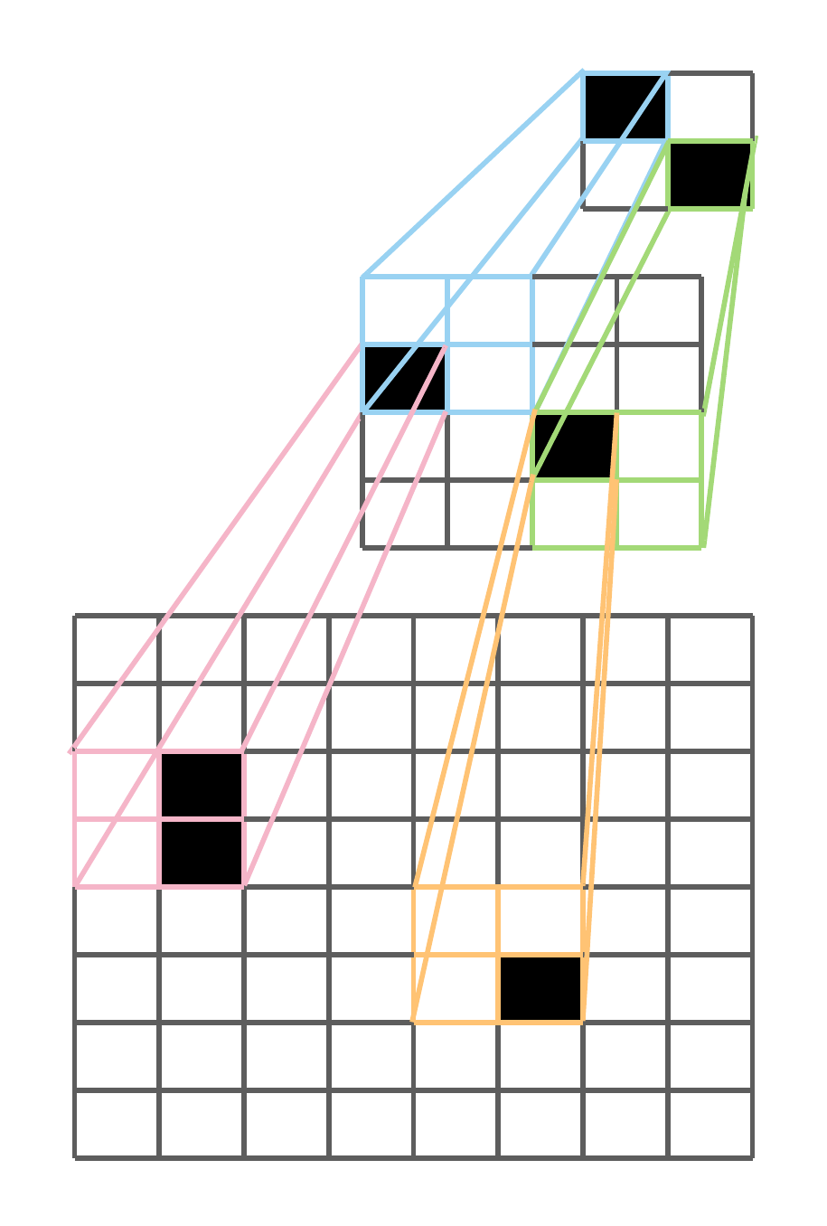
the corresponding point_hierarchies would be:
>>> torch.ShortTensor([[0, 0], [1, 1],
                       [1, 0], [2, 2],
                       [2, 1], [3, 1], [5, 5]
                      ])
Note
To generate points see kaolin.ops.generate_points()
Note
the tensors pyramid, exsum and points are used by many Structured Point Cloud functions; avoiding their recomputation will improve performace.
Convolutions
We provide several sparse convolution layers for structured point clouds.
Convolutions are characterized by the size of the input and output channels,
an array of kernel_vectors, and possibly the number of levels to jump, i.e.,
the difference in input and output levels.
An example of how to create a \(3 \times 3 \times 3\) kernel follows:
>>> vectors = []
>>> for i in range(-1, 2):
>>>     for j in range(-1, 2):
>>>         for k in range(-1, 2):
>>>             vectors.append([i, j, k])
>>> Kvec = torch.tensor(vectors, dtype=torch.short, device=device)
>>> Kvec
tensor([[-1, -1, -1],
        [-1, -1,  0],
        [-1, -1,  1],
        ...
        ...
        [ 1,  1, -1],
        [ 1,  1,  0],
        [ 1,  1,  1]], device='cuda:0', dtype=torch.int16)
The kernel vectors determine the shape of the convolution kernel. Each kernel vector is added to the position of a point to determine the coordinates of points whose corresponding input data is needed for the operation. We formalize this notion using the following neighbor function:
that returns the index of the point within the same level found by adding kernel vector \(\overrightarrow{K}_k\) to point \(P_i\). Given the sparse nature of SPC data, it may be the case that no such point exists. In such cases, \(n(i,k)\) will return an invalid value, and data accesses will be treated like zero padding.
Transposed convolutions are defined by the transposed neighbor function
The value jump is used to indicate the difference in levels between the iput features and the output features. For convolutions, this is the number of levels to downsample; while for transposed convolutions, jump is the number of levels to upsample. The value of jump must be positive, and may not go beyond the highest level of the octree.
Examples
You can create octrees from sparse feature_grids (of shape \((\text{batch_size}, \text{feature_dim}, \text{height}, \text{width}, \text{depth})\)):
>>> octrees, lengths, features = kaolin.ops.spc.feature_grids_to_spc(features_grids)
or from point cloud (of shape \((\text{num_points, 3})\)):
>>> qpc = kaolin.ops.spc.quantize_points(pc, level)
>>> octree = kaolin.ops.spc.unbatched_points_to_octree(qpc, level)
To use convolution, you can use the functional or the torch.nn.Module version like torch.nn.functional.conv3d and torch.nn.Conv3d:
>>> max_level, pyramids, exsum = kaolin.ops.spc.scan_octrees(octrees, lengths)
>>> point_hierarchies = kaolin.ops.spc.generate_points(octrees, pyramids, exsum)
>>> kernel_vectors = torch.tensor([[0, 0, 0], [0, 0, 1], [0, 1, 0], [0, 1, 1],
                                   [1, 0, 0], [1, 0, 1], [1, 1, 0], [1, 1, 1]],
                                  dtype=torch.ShortTensor, device='cuda')
>>> conv = kaolin.ops.spc.Conv3d(in_channels, out_channels, kernel_vectors, jump=1, bias=True).cuda()
>>> # With functional
>>> out_features, out_level = kaolin.ops.spc.conv3d(octrees, point_hierarchies, level, pyramids,
...                                                 exsum, coalescent_features, weight,
...                                                 kernel_vectors, jump, bias)
>>> # With nn.Module and container class
>>> input_spc = kaolin.rep.Spc(octrees, lengths)
>>> conv
>>> out_features, out_level = kaolin.ops.spc.conv_transpose3d(
...     **input_spc.to_dict(), input=out_features, level=level,
...     weight=weight, kernel_vectors=kernel_vectors, jump=jump, bias=bias)
To apply ray tracing we currently only support non-batched version, for instance here with RGB values as per point features:
>>> max_level, pyramids, exsum = kaolin.ops.spc.scan_octrees(
...     octree, torch.tensor([len(octree)], dtype=torch.int32, device='cuda')
>>> point_hierarchy = kaolin.ops.spc.generate_points(octrees, pyramids, exsum)
>>> ridx, pidx, depth = kaolin.render.spc.unbatched_raytrace(octree, point_hierarchy, pyramids[0], exsum,
...                                                          origin, direction, max_level)
>>> first_hits_mask = kaolin.render.spc.mark_pack_boundaries(ridx)
>>> first_hits_point = pidx[first_hits_mask]
>>> first_hits_rgb = rgb[first_hits_point - pyramids[max_level - 2]]
Going further with SPC:
Examples:
See our Jupyter notebook for a walk-through of SPC features:
examples/tutorial/understanding_spcs_tutorial.ipynb
And also our recipes for simple examples of how to use SPC:
spc_basics.py: showing attributes of an SPC object
spc_dual_octree.py: computing and explaining the dual of an SPC octree
spc_trilinear_interp.py: computing trilinear interpolation of a point cloud on an SPC
SPC Documentation:
Functions useful for working with SPCs are available in the following modules:
kaolin.ops.spc - general explanation and operations
kaolin.render.spc - rendering utilities
kaolin.rep.Spc- high-level wrapper.. _kaolin.ops.spc: